利用 CNN 來預測數字 (MNIST)
輸入圖形是一個 2828 灰階 0~9 的數字。輸出是一個 110 的矩陣,代表預測 0~9 的機率分布。
流程如下:
輸入 – convolution – pooling – convolution – pooling – hidden layer – output
在代碼中用到 [None, xx, xx] 和 [-1, XX, xx],代表我們忽略輸入的大小(batch size),它會跟隨著輸入自動改變。
max pooling 表示我們選擇的是那個 kernel size 裡的最大值。結構中也加入了 dropout 來避免 overfitting。
完整的程式如下:
import tensorflow as tf
from tensorflow.examples.tutorials.mnist import input_data
# input and datatype
mnist = input_data.read_data_sets("MNIST_data/", one_hot = True)
x_ = tf.placeholder(tf.float32, [None,784])  ##28*28
y_ = tf.placeholder(tf.float32, [None,10])
x_image = tf.reshape(x_, [-1,28,28,1])  ## Gray scale:1  RBG:3
keep_prob = tf.placeholder(tf.float32)

# define W, b convolution
def Weight_variable(shape):
    initial = tf.truncated_normal(shape, stddev=0.1)
    return tf.Variable(initial)

def bias_variable(shape):
    initial = tf.constant(0.12, shape=shape)
    return tf.Variable(initial)

def conv2d(x, W):
    return tf.nn.conv2d(x, W, [1,1,1,1],padding='SAME')

def max_pool_2x2(x):
    return tf.nn.max_pool(x, ksize=[1,2,2,1], strides=[1,2,2,1],padding='SAME')

# con1 use 5*5  1 to 32
W_conv1 = Weight_variable([5,5,1,32])
b_conv1 = bias_variable([32])
hidden_conv1 = tf.nn.relu(conv2d(x_image, W_conv1) + b_conv1)
hidden_pool1 = max_pool_2x2(hidden_conv1)
# con2
W_conv2 = Weight_variable([5,5,32,64])
b_conv2 = bias_variable([64])
hidden_conv2 = tf.nn.relu(conv2d(hidden_pool1, W_conv2) + b_conv2)
hidden_pool2 = max_pool_2x2(hidden_conv2)

# hidden layer 1   28*28 -- 14*14 -- 7*7
hidden_x1 = tf.reshape(hidden_pool2, [-1, 7*7*64])
hidden_W1 = Weight_variable([7*7*64, 512])
hidden_b1 = bias_variable([512])
hidden_act1 = tf.nn.relu(tf.matmul(hidden_x1, hidden_W1) + hidden_b1)
# dropout
hidden_drop = tf.nn.dropout(hidden_act1, keep_prob)
# output layer
prediction_W = Weight_variable([512,10])
prediction_b = bias_variable([10])
prediction = tf.nn.softmax(tf.matmul(hidden_drop, prediction_W) + prediction_b)
# [True, False, False, False, False] = [1, 0, 0, 0, 0] = 0.2
def compute_accuracy(v_xs, v_ys):
    global prediction
    y_prediction = sess.run(prediction, {x_:v_xs, keep_prob:1})
    correct_prediction = tf.equal(tf.argmax(y_prediction,1), tf.argmax(v_ys,1))
    accuracy = tf.reduce_mean(tf.cast(correct_prediction,tf.float32))
    # result  = sess.run(accuracy, {x_: v_xs, y_:v_ys keep_prob:1})
    result = accuracy.eval({x_: v_xs, y_:v_ys, keep_prob:1})
    return result
# cross_entropy
cross_entropy = tf.reduce_mean(-tf.reduce_sum(y_ * tf.log(prediction),
                               reduction_indices=[1]))
tf.summary.scalar('loss', cross_entropy)
train_step = tf.train.GradientDescentOptimizer(0.02).minimize(cross_entropy)
# initial
sess = tf.InteractiveSession(config=tf.ConfigProto(log_device_placement=True))
tf.global_variables_initializer().run()
merged = tf.summary.merge_all()
train_writer = tf.summary.FileWriter("./train", sess.graph)
test_writer = tf.summary.FileWriter("./test", sess.graph)
##sess.run(tf.global_variables_initializer())

# train
for i in range(1000):
    batch = mnist.train.next_batch(100) ##Stochastic gradient descent
    sess.run(train_step, feed_dict={x_:batch[0], y_:batch[1], keep_prob:0.8})
    if i %50==0:
        print(compute_accuracy(mnist.test.images,mnist.test.labels))
        train_result = sess.run(merged, {x_:batch[0], y_:batch[1], keep_prob: 1})
        test_result = sess.run(merged, {x_:mnist.test.images, y_:mnist.test.labels,
                                         keep_prob: 1})
        train_writer.add_summary(train_result, i)
        test_writer.add_summary(test_result, i)
結果
上圖是沒有 dropout,下圖是有 dropout。就這個例子而言差別不大,但還是看得出來上面的訓練會比測試好。
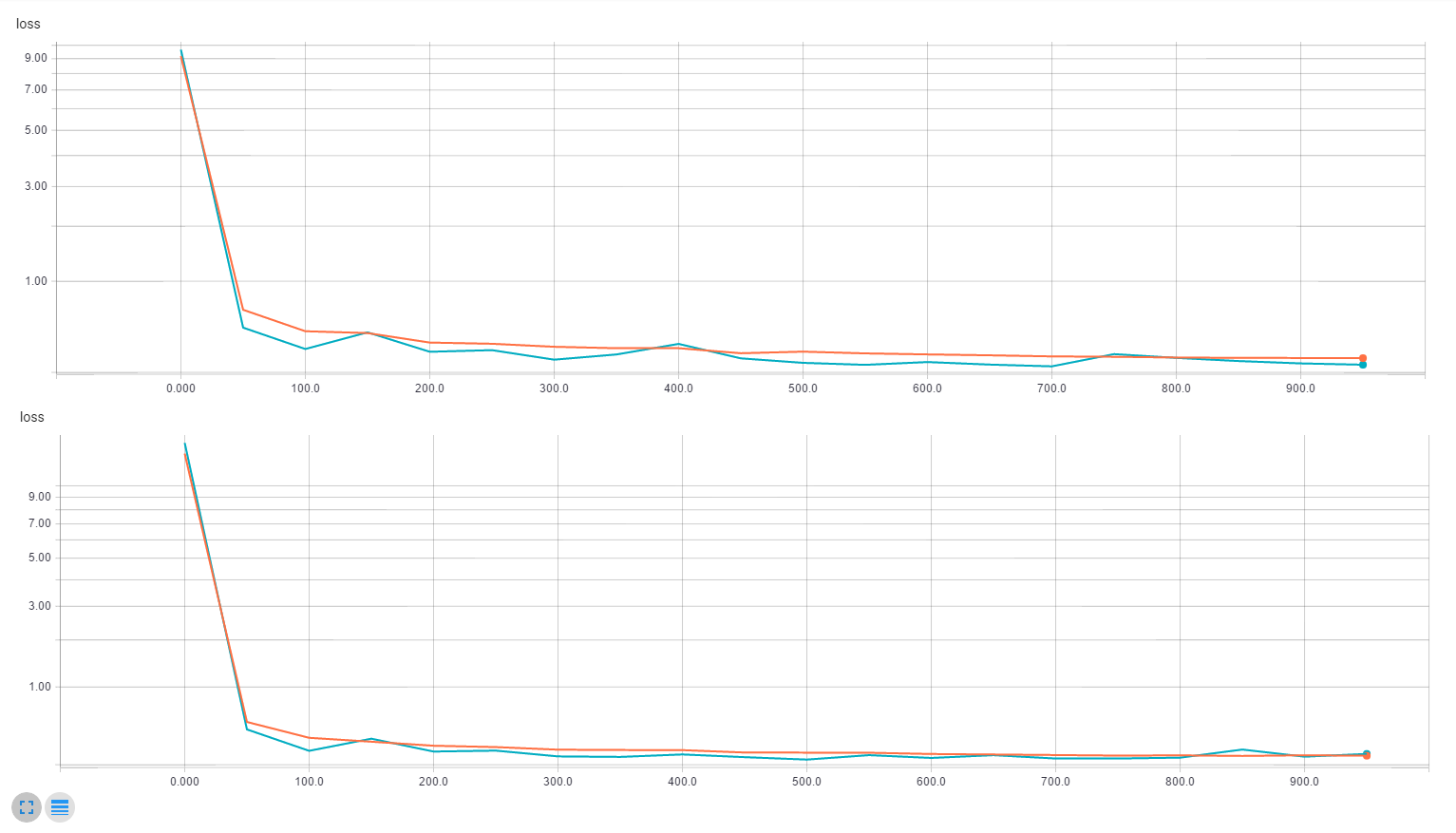
準確率落在 97%~99% 之間 (1000 次訓練)。
(目前使用 GradientDescent,更換優化器應該會更好)。